Hello PyTorch

13 minute read

Published: September 14, 2024

The objective is to use the very basic example of linear regression and use PyTorch to build a model to demonstrate Pytorch workflow and its fundementals.

I will develop a simple model using Pytorch and they use a layered NN to perform the same prediction.

import torch
from torch import nn
import matplotlib.pyplot as plt
torch.__version__

'2.4.1+cu121'

Simple linear regression problem

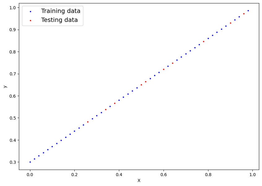
I will use the freecodecamp example which I find very usefull to get into the fundementals. This will try to build a model which trains 2 variables; Bias and weight of a line. We will generate sample data with predefined values of .3 and .7 and train the model based on the sample data which we have generated.

generate sample data

# We will generate data based on the predefined weight and bias. this will generate a sample set of 5 values
weight = .7
bias = .3
start = 0
end = 1
step = .02
X = torch.arange(start, end, step).unsqueeze(dim=1)
print(X.shape)
y = weight * X + bias
X[:5] , y[:5]

torch.Size([50, 1])





(tensor([[0.0000],
         [0.0200],
         [0.0400],
         [0.0600],
         [0.0800]]),
 tensor([[0.3000],
         [0.3140],
         [0.3280],
         [0.3420],
         [0.3560]]))

# prompt: split the data X and y for train and test at random positions

from sklearn.model_selection import train_test_split

X_train, X_test, y_train, y_test = train_test_split(
    X, y, test_size=0.2, random_state=42
)

print(f"X_train shape: {X_train.shape}")
print(f"y_train shape: {y_train.shape}")
print(f"X_test shape: {X_test.shape}")
print(f"y_test shape: {y_test.shape}")

X_train shape: torch.Size([40, 1])
y_train shape: torch.Size([40, 1])
X_test shape: torch.Size([10, 1])
y_test shape: torch.Size([10, 1])

Visualize the sample data

# prompt: visualize the X_train, X_test, y_train, y_test

plt.figure(figsize=(10, 7))
plt.scatter(X_train, y_train, c="b", s=4, label="Training data")
plt.scatter(X_test, y_test, c="r", s=4, label="Testing data")
plt.legend(fontsize=14)
plt.xlabel("X")
plt.ylabel("y")
plt.show()

Model Development

So we need to build a model close to the above line and test the model on the red dots and get a result as close to it.

This is developed by inheriting the nn.Module class

Step 1 : initialize the paramters of bias and weight to a random value

Step 2 : Build a model using a custom funcion = X * weight + Bias.

class LinearRegressionModelKFN(nn.Module):
    # The objective is to start with a random weight and bias and then usen the pytorch to figure out the best value based on the training data.
    # This is done either by gradient decent or Back propogation.
    # we have set requires_grad=True

    def __init__(self):
        super().__init__()
        self.weight = nn.Parameter(torch.randn(1, requires_grad=True, dtype=torch.float))
        self.bias = nn.Parameter(torch.randn(1, requires_grad=True, dtype=torch.float))

    # we need to overide the forward method
    def forward(self, x: torch.Tensor) -> torch.Tensor:
        return self.weight * x + self.bias

Initial random values of our model

torch.manual_seed(42)
model_0 = LinearRegressionModelKFN()
print(list(model_0.parameters()))
print(model_0.state_dict())
with torch.inference_mode():
    y_preds = model_0(X_test)

y_preds

[Parameter containing:
tensor([0.3367], requires_grad=True), Parameter containing:
tensor([0.1288], requires_grad=True)]
OrderedDict([('weight', tensor([0.3367])), ('bias', tensor([0.1288]))])





tensor([[0.2163],
        [0.3914],
        [0.3308],
        [0.4318],
        [0.2433],
        [0.4520],
        [0.3039],
        [0.2972],
        [0.3443],
        [0.2568]])

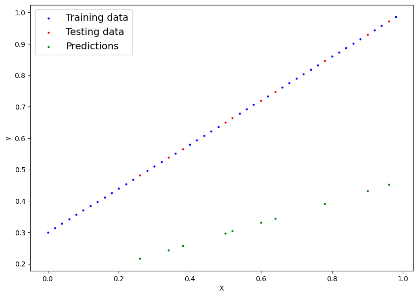
Ploting the initial model with random parameters

We need to use pytorch to bring the green line as close to the red line

# prompt: add to the plt the y_preds

plt.figure(figsize=(10, 7))
plt.scatter(X_train, y_train, c="b", s=4, label="Training data")
plt.scatter(X_test, y_test, c="r", s=4, label="Testing data")
plt.scatter(X_test, y_preds, c="g",  s=4, label="Predictions")
plt.legend(fontsize=14)
plt.xlabel("X")
plt.ylabel("y")
plt.show()

Pytorch Workflow

We will define a loss function and a optimizer and iteratively use them to enhance the model by reducing the loss function.

We will also track the progress of the loss function

# prompt: set a lossfunction using L1Loss and a Optimizer using SGD
loss_fn = nn.L1Loss()
optimizer = torch.optim.SGD(params = model_0.parameters(), lr=0.001)

# variable as used to iterate the number of time.
epochs = 1500

# Below variables are used to track the progress
epoch_values = []
loss_values = []
test_loss_values = []

# Workflow
for epoch in range(epochs):
    # set the model into training mode
    model_0.train()

    # Step 1: Forward Pass
    y_preds = model_0(X_train)

    # Step 2: Calculate the loss
    loss = loss_fn(y_preds, y_train)

    # Step 3: Opimizer zero grad to reset every loop
    optimizer.zero_grad()

    # Step 4: Perform back propogation
    loss.backward()

    # Step 5: Step the optimizer
    optimizer.step()


    # Progress tracking
    if epoch % 100 == 0:
      print(f"Epoch: {epoch} | Loss: {loss}")
      model_0.eval()
      print(model_0.state_dict())
      with torch.inference_mode():
        test_preds = model_0(X_test)
        test_loss = loss_fn(test_preds, y_test)
      epoch_values.append(epoch)
      loss_values.append(loss.detach().numpy())
      test_loss_values.append(test_loss.detach().numpy())

Epoch: 0 | Loss: 0.340311199426651
OrderedDict([('weight', tensor([0.3372])), ('bias', tensor([0.1298]))])
Epoch: 100 | Loss: 0.21864144504070282
OrderedDict([('weight', tensor([0.3837])), ('bias', tensor([0.2298]))])
Epoch: 200 | Loss: 0.10451823472976685
OrderedDict([('weight', tensor([0.4301])), ('bias', tensor([0.3256]))])
Epoch: 300 | Loss: 0.06448396295309067
OrderedDict([('weight', tensor([0.4709])), ('bias', tensor([0.3713]))])
Epoch: 400 | Loss: 0.05163732171058655
OrderedDict([('weight', tensor([0.5030])), ('bias', tensor([0.3857]))])
Epoch: 500 | Loss: 0.045265451073646545
OrderedDict([('weight', tensor([0.5278])), ('bias', tensor([0.3827]))])
Epoch: 600 | Loss: 0.03966418653726578
OrderedDict([('weight', tensor([0.5492])), ('bias', tensor([0.3727]))])
Epoch: 700 | Loss: 0.03406292945146561
OrderedDict([('weight', tensor([0.5707])), ('bias', tensor([0.3627]))])
Epoch: 800 | Loss: 0.028461668640375137
OrderedDict([('weight', tensor([0.5921])), ('bias', tensor([0.3527]))])
Epoch: 900 | Loss: 0.02286040410399437
OrderedDict([('weight', tensor([0.6136])), ('bias', tensor([0.3427]))])
Epoch: 1000 | Loss: 0.0172591470181942
OrderedDict([('weight', tensor([0.6351])), ('bias', tensor([0.3327]))])
Epoch: 1100 | Loss: 0.011657887138426304
OrderedDict([('weight', tensor([0.6565])), ('bias', tensor([0.3227]))])
Epoch: 1200 | Loss: 0.006066909525543451
OrderedDict([('weight', tensor([0.6776])), ('bias', tensor([0.3121]))])
Epoch: 1300 | Loss: 0.0004846327065024525
OrderedDict([('weight', tensor([0.6984])), ('bias', tensor([0.3009]))])
Epoch: 1400 | Loss: 0.00019141807570122182
OrderedDict([('weight', tensor([0.7002])), ('bias', tensor([0.3009]))])

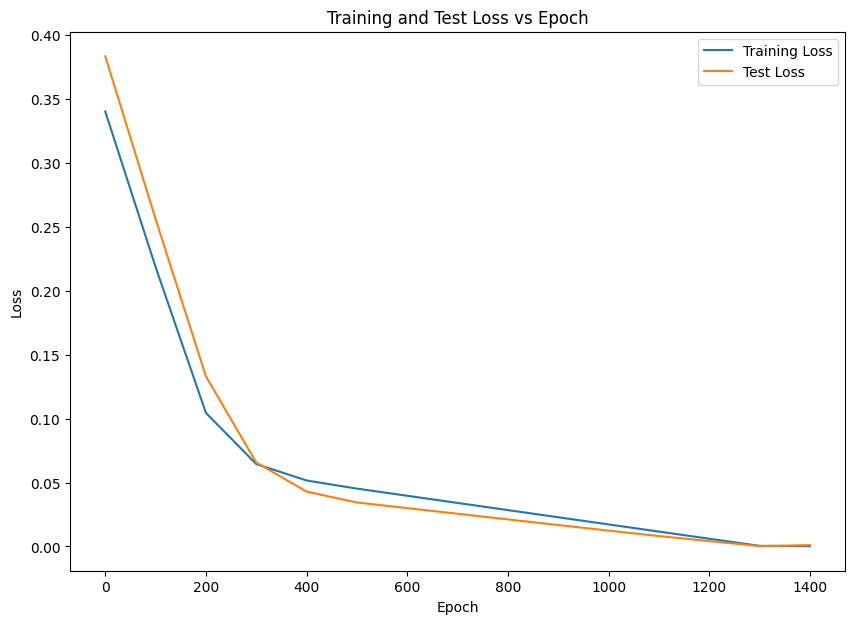
Plotting the progress tracking

# prompt: Plot to compare epoch_values with loss_values and test_loss_values

plt.figure(figsize=(10, 7))
plt.plot(epoch_values, loss_values, label="Training Loss")
plt.plot(epoch_values, test_loss_values, label="Test Loss")
plt.xlabel("Epoch")
plt.ylabel("Loss")
plt.title("Training and Test Loss vs Epoch")
plt.legend()
plt.show()

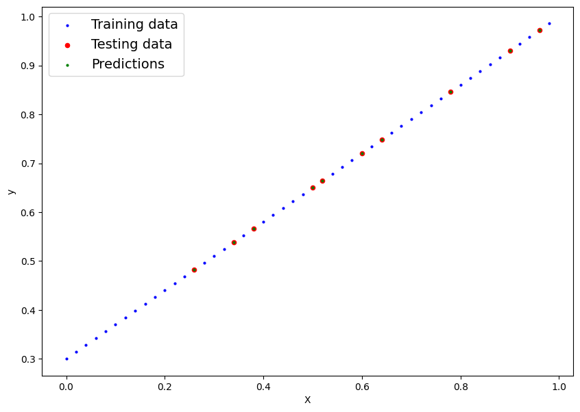
Plotting the model output predictions

# prompt: plot the new y_preds along with the Xtrain and X test
model_0.eval()
print(model_0.state_dict())
with torch.inference_mode():
    y_preds = model_0(X_test)

plt.figure(figsize=(10, 7))
plt.scatter(X_train, y_train, c="b", s=4, label="Training data")
plt.scatter(X_test, y_test, c="r", s=20, label="Testing data")
plt.scatter(X_test, y_preds, c="g",  s=4, label="Predictions")
plt.legend(fontsize=14)
plt.xlabel("X")
plt.ylabel("y")
plt.show()

OrderedDict([('weight', tensor([0.6998])), ('bias', tensor([0.2999]))])

2 layered NN

# prompt: Create a new model which will perform the same but using a 2 layered nueral network


# Define a two-layer linear regression model
class LinearRegressionModelKFN2Layer(nn.Module):
    def __init__(self):
        """
        Constructor for the LinearRegressionModelKFN2Layer class. This initializes a simple neural 
        network with two linear layers. The first linear layer transforms the input with one feature 
        into a hidden layer with 10 neurons. The second linear layer transforms the hidden layer's 
        output into a single value (the predicted output).
        """
        super().__init__()
        
        # Define the first linear layer (input layer), which takes 1 feature and outputs 10 neurons
        self.linear1 = nn.Linear(1, 10)
        
        # Define the second linear layer (output layer), which takes 10 neurons as input and outputs 1 value
        self.linear2 = nn.Linear(10, 1)

    def forward(self, x):
        """
        Forward pass through the neural network. This method takes the input `x`, applies the first
        linear transformation, passes it through the ReLU activation function, and then applies the
        second linear transformation to get the output.

        Args:
        x (Tensor): Input tensor containing the feature(s), where each row is an example and 
                    each column is a feature (for this case, there is 1 feature per example).

        Returns:
        Tensor: The output of the model, which is the predicted value.
        """
        # Apply the first linear layer, followed by a ReLU activation function
        x = torch.relu(self.linear1(x))
        
        # Apply the second linear layer to get the final output (predicted value)
        x = self.linear2(x)
        
        return x
torch.manual_seed(42)
model_2layer = LinearRegressionModelKFN2Layer()
print(list(model_2layer.parameters()))
print(model_2layer.state_dict())

OrderedDict([('linear1.weight', tensor([[ 0.7645],
        [ 0.8300],
        [-0.2343],
        [ 0.9186],
        [-0.2191],
        [ 0.2018],
        [-0.4869],
        [ 0.5873],
        [ 0.8815],
        [-0.7336]])), ('linear1.bias', tensor([ 0.8692,  0.1872,  0.7388,  0.1354,  0.4822, -0.1412,  0.7709,  0.1478,
        -0.4668,  0.2549])), ('linear2.weight', tensor([[-0.1457, -0.0371, -0.1284,  0.2098, -0.2496, -0.1458, -0.0893, -0.1901,
          0.0298, -0.3123]])), ('linear2.bias', tensor([0.2856]))])

with torch.inference_mode():
    y_preds = model_2layer(X_test)

y_preds

# ### Ploting the initial model with random parameters
# 
# We need to use pytorch to bring the green line as close to the red line

plt.figure(figsize=(10, 7))
plt.scatter(X_train, y_train, c="b", s=4, label="Training data")
plt.scatter(X_test, y_test, c="r", s=4, label="Testing data")
plt.scatter(X_test, y_preds, c="g",  s=4, label="Predictions")
plt.legend(fontsize=14)
plt.xlabel("X")
plt.ylabel("y")
plt.show()

# ## Pytorch Workflow
# 
# We will define a loss function and a optimizer and iteratively use them to enhance the model by reducing the loss function.
# 
# We will also track the progress of the loss function
loss_fn = nn.L1Loss()
optimizer = torch.optim.SGD(params = model_2layer.parameters(), lr=0.001)

# variable as used to iterate the number of time.
epochs = 1500

# Below variables are used to track the progress
epoch_values = []
loss_values = []
test_loss_values = []

# Workflow
for epoch in range(epochs):
    # set the model into training mode
    model_2layer.train()

    # Step 1: Forward Pass
    y_preds = model_2layer(X_train)

    # Step 2: Calculate the loss
    loss = loss_fn(y_preds, y_train)

    # Step 3: Opimizer zero grad to reset every loop
    optimizer.zero_grad()

    # Step 4: Perform back propogation
    loss.backward()

    # Step 5: Step the optimizer
    optimizer.step()


    # Progress tracking
    if epoch % 100 == 0:
      print(f"Epoch: {epoch} | Loss: {loss}")
      model_2layer.eval()
      print(model_2layer.state_dict())
      with torch.inference_mode():
        test_preds = model_2layer(X_test)
        test_loss = loss_fn(test_preds, y_test)
      epoch_values.append(epoch)
      loss_values.append(loss.detach().numpy())
      test_loss_values.append(test_loss.detach().numpy())

# ### Plotting the progress tracking

plt.figure(figsize=(10, 7))
plt.plot(epoch_values, loss_values, label="Training Loss")
plt.plot(epoch_values, test_loss_values, label="Test Loss")
plt.xlabel("Epoch")
plt.ylabel("Loss")
plt.title("Training and Test Loss vs Epoch")
plt.legend()
plt.show()

# Plotting the model output predictions
model_2layer.eval()
print(model_2layer.state_dict())
with torch.inference_mode():
    y_preds = model_2layer(X_test)

plt.figure(figsize=(10, 7))
plt.scatter(X_train, y_train, c="b", s=4, label="Training data")
plt.scatter(X_test, y_test, c="r", s=20, label="Testing data")
plt.scatter(X_test, y_preds, c="g",  s=4, label="Predictions")
plt.legend(fontsize=14)
plt.xlabel("X")
plt.ylabel("y")
plt.show()

        Epoch: 0 | Loss: 0.7426110506057739
  OrderedDict([('linear1.weight', tensor([[ 0.7645],
          [ 0.8300],
          [-0.2343],
          [ 0.9187],
          [-0.2192],
          [ 0.2018],
          [-0.4869],
          [ 0.5872],
          [ 0.8816],
          [-0.7336]])), ('linear1.bias', tensor([ 0.8691,  0.1871,  0.7387,  0.1356,  0.4819, -0.1412,  0.7708,  0.1476,
          -0.4668,  0.2548])), ('linear2.weight', tensor([[-0.1445, -0.0365, -0.1278,  0.2103, -0.2492, -0.1458, -0.0888, -0.1897,
            0.0299, -0.3123]])), ('linear2.bias', tensor([0.2866]))])
  Epoch: 100 | Loss: 0.3070870339870453
  OrderedDict([('linear1.weight', tensor([[ 0.7606],
          [ 0.8296],
          [-0.2388],
          [ 0.9298],
          [-0.2300],
          [ 0.1985],
          [-0.4898],
          [ 0.5793],
          [ 0.8827],
          [-0.7356]])), ('linear1.bias', tensor([ 0.8606,  0.1863,  0.7290,  0.1595,  0.4588, -0.1451,  0.7646,  0.1307,
          -0.4653,  0.2424])), ('linear2.weight', tensor([[-0.0226,  0.0207, -0.0655,  0.2680, -0.2127, -0.1451, -0.0348, -0.1487,
            0.0390, -0.3068]])), ('linear2.bias', tensor([0.3866]))])
  Epoch: 200 | Loss: 0.06249262019991875
  OrderedDict([('linear1.weight', tensor([[ 0.7616],
          [ 0.8314],
          [-0.2406],
          [ 0.9416],
          [-0.2381],
          [ 0.1956],
          [-0.4904],
          [ 0.5740],
          [ 0.8842],
          [-0.7358]])), ('linear1.bias', tensor([ 0.8615,  0.1886,  0.7262,  0.1766,  0.4467, -0.1485,  0.7634,  0.1225,
          -0.4633,  0.2418])), ('linear2.weight', tensor([[ 0.0595,  0.0654, -0.0317,  0.3158, -0.1951, -0.1445, -0.0089, -0.1178,
            0.0481, -0.3070]])), ('linear2.bias', tensor([0.4463]))])
  Epoch: 300 | Loss: 0.04238714650273323
  OrderedDict([('linear1.weight', tensor([[ 0.7631],
          [ 0.8331],
          [-0.2414],
          [ 0.9491],
          [-0.2426],
          [ 0.1930],
          [-0.4908],
          [ 0.5714],
          [ 0.8860],
          [-0.7339]])), ('linear1.bias', tensor([ 0.8610,  0.1881,  0.7264,  0.1744,  0.4481, -0.1514,  0.7636,  0.1233,
          -0.4610,  0.2542])), ('linear2.weight', tensor([[ 0.0711,  0.0832, -0.0422,  0.3363, -0.2036, -0.1441, -0.0254, -0.1056,
            0.0574, -0.3124]])), ('linear2.bias', tensor([0.4395]))])
  Epoch: 400 | Loss: 0.02345609851181507
  OrderedDict([('linear1.weight', tensor([[ 0.7647],
          [ 0.8351],
          [-0.2424],
          [ 0.9565],
          [-0.2471],
          [ 0.1906],
          [-0.4915],
          [ 0.5693],
          [ 0.8881],
          [-0.7319]])), ('linear1.bias', tensor([ 0.8602,  0.1871,  0.7269,  0.1709,  0.4502, -0.1541,  0.7639,  0.1243,
          -0.4582,  0.2670])), ('linear2.weight', tensor([[ 0.0789,  0.0992, -0.0547,  0.3550, -0.2134, -0.1438, -0.0436, -0.0946,
            0.0669, -0.3183]])), ('linear2.bias', tensor([0.4295]))])
  Epoch: 500 | Loss: 0.011140111833810806
  OrderedDict([('linear1.weight', tensor([[ 0.7661],
          [ 0.8368],
          [-0.2434],
          [ 0.9625],
          [-0.2507],
          [ 0.1885],
          [-0.4924],
          [ 0.5678],
          [ 0.8901],
          [-0.7297]])), ('linear1.bias', tensor([ 0.8597,  0.1864,  0.7273,  0.1684,  0.4517, -0.1565,  0.7643,  0.1249,
          -0.4556,  0.2766])), ('linear2.weight', tensor([[ 0.0856,  0.1118, -0.0637,  0.3697, -0.2206, -0.1436, -0.0570, -0.0860,
            0.0761, -0.3215]])), ('linear2.bias', tensor([0.4226]))])
  Epoch: 600 | Loss: 0.009158110246062279
  OrderedDict([('linear1.weight', tensor([[ 0.7665],
          [ 0.8374],
          [-0.2438],
          [ 0.9645],
          [-0.2518],
          [ 0.1867],
          [-0.4927],
          [ 0.5673],
          [ 0.8914],
          [-0.7283]])), ('linear1.bias', tensor([ 0.8594,  0.1861,  0.7275,  0.1673,  0.4524, -0.1584,  0.7644,  0.1252,
          -0.4545,  0.2782])), ('linear2.weight', tensor([[ 0.0870,  0.1156, -0.0672,  0.3743, -0.2233, -0.1434, -0.0619, -0.0834,
            0.0832, -0.3196]])), ('linear2.bias', tensor([0.4195]))])
  Epoch: 700 | Loss: 0.008464774116873741
  OrderedDict([('linear1.weight', tensor([[ 0.7666],
          [ 0.8376],
          [-0.2439],
          [ 0.9650],
          [-0.2522],
          [ 0.1852],
          [-0.4928],
          [ 0.5672],
          [ 0.8922],
          [-0.7273]])), ('linear1.bias', tensor([ 0.8593,  0.1859,  0.7276,  0.1668,  0.4527, -0.1601,  0.7645,  0.1253,
          -0.4539,  0.2768])), ('linear2.weight', tensor([[ 0.0870,  0.1166, -0.0685,  0.3754, -0.2243, -0.1432, -0.0636, -0.0828,
            0.0891, -0.3161]])), ('linear2.bias', tensor([0.4182]))])
  Epoch: 800 | Loss: 0.007900995202362537
  OrderedDict([('linear1.weight', tensor([[ 0.7667],
          [ 0.8376],
          [-0.2439],
          [ 0.9652],
          [-0.2522],
          [ 0.1838],
          [-0.4928],
          [ 0.5672],
          [ 0.8930],
          [-0.7265]])), ('linear1.bias', tensor([ 0.8593,  0.1859,  0.7276,  0.1666,  0.4528, -0.1615,  0.7646,  0.1253,
          -0.4535,  0.2745])), ('linear2.weight', tensor([[ 0.0868,  0.1168, -0.0690,  0.3757, -0.2246, -0.1431, -0.0642, -0.0826,
            0.0945, -0.3122]])), ('linear2.bias', tensor([0.4177]))])
  Epoch: 900 | Loss: 0.007354866713285446
  OrderedDict([('linear1.weight', tensor([[ 0.7667],
          [ 0.8376],
          [-0.2439],
          [ 0.9652],
          [-0.2523],
          [ 0.1828],
          [-0.4928],
          [ 0.5672],
          [ 0.8938],
          [-0.7257]])), ('linear1.bias', tensor([ 0.8592,  0.1858,  0.7277,  0.1664,  0.4529, -0.1626,  0.7646,  0.1254,
          -0.4530,  0.2722])), ('linear2.weight', tensor([[ 0.0865,  0.1169, -0.0694,  0.3758, -0.2249, -0.1430, -0.0647, -0.0826,
            0.0999, -0.3083]])), ('linear2.bias', tensor([0.4171]))])
  Epoch: 1000 | Loss: 0.00681077316403389
  OrderedDict([('linear1.weight', tensor([[ 0.7667],
          [ 0.8377],
          [-0.2439],
          [ 0.9654],
          [-0.2524],
          [ 0.1818],
          [-0.4928],
          [ 0.5671],
          [ 0.8947],
          [-0.7249]])), ('linear1.bias', tensor([ 0.8592,  0.1857,  0.7277,  0.1662,  0.4530, -0.1637,  0.7646,  0.1254,
          -0.4526,  0.2699])), ('linear2.weight', tensor([[ 0.0863,  0.1170, -0.0699,  0.3760, -0.2252, -0.1430, -0.0653, -0.0825,
            0.1053, -0.3044]])), ('linear2.bias', tensor([0.4166]))])
  Epoch: 1100 | Loss: 0.006268690340220928
  OrderedDict([('linear1.weight', tensor([[ 0.7667],
          [ 0.8377],
          [-0.2439],
          [ 0.9654],
          [-0.2524],
          [ 0.1808],
          [-0.4928],
          [ 0.5671],
          [ 0.8956],
          [-0.7241]])), ('linear1.bias', tensor([ 0.8591,  0.1857,  0.7277,  0.1660,  0.4531, -0.1648,  0.7647,  0.1255,
          -0.4521,  0.2676])), ('linear2.weight', tensor([[ 0.0860,  0.1171, -0.0703,  0.3762, -0.2255, -0.1429, -0.0658, -0.0824,
            0.1107, -0.3006]])), ('linear2.bias', tensor([0.4161]))])
  Epoch: 1200 | Loss: 0.005730263888835907
  OrderedDict([('linear1.weight', tensor([[ 0.7667],
          [ 0.8377],
          [-0.2440],
          [ 0.9655],
          [-0.2525],
          [ 0.1798],
          [-0.4928],
          [ 0.5671],
          [ 0.8965],
          [-0.7234]])), ('linear1.bias', tensor([ 0.8591,  0.1856,  0.7278,  0.1658,  0.4533, -0.1658,  0.7647,  0.1255,
          -0.4516,  0.2654])), ('linear2.weight', tensor([[ 0.0857,  0.1172, -0.0708,  0.3763, -0.2258, -0.1429, -0.0663, -0.0823,
            0.1161, -0.2967]])), ('linear2.bias', tensor([0.4155]))])
  Epoch: 1300 | Loss: 0.005442876368761063
  OrderedDict([('linear1.weight', tensor([[ 0.7667],
          [ 0.8377],
          [-0.2439],
          [ 0.9653],
          [-0.2523],
          [ 0.1791],
          [-0.4928],
          [ 0.5671],
          [ 0.8974],
          [-0.7227]])), ('linear1.bias', tensor([ 0.8591,  0.1856,  0.7278,  0.1657,  0.4533, -0.1665,  0.7647,  0.1255,
          -0.4511,  0.2630])), ('linear2.weight', tensor([[ 0.0851,  0.1166, -0.0707,  0.3757, -0.2257, -0.1429, -0.0661, -0.0827,
            0.1208, -0.2928]])), ('linear2.bias', tensor([0.4154]))])
  Epoch: 1400 | Loss: 0.00519354036077857
  OrderedDict([('linear1.weight', tensor([[ 0.7666],
          [ 0.8375],
          [-0.2438],
          [ 0.9649],
          [-0.2521],
          [ 0.1785],
          [-0.4927],
          [ 0.5672],
          [ 0.8983],
          [-0.7218]])), ('linear1.bias', tensor([ 0.8591,  0.1856,  0.7278,  0.1658,  0.4532, -0.1672,  0.7647,  0.1255,
          -0.4502,  0.2613])), ('linear2.weight', tensor([[ 0.0847,  0.1159, -0.0703,  0.3748, -0.2253, -0.1428, -0.0654, -0.0832,
            0.1242, -0.2893]])), ('linear2.bias', tensor([0.4157]))])

OrderedDict([('linear1.weight', tensor([[ 0.7666],
        [ 0.8375],
        [-0.2438],
        [ 0.9649],
        [-0.2521],
        [ 0.1780],
        [-0.4927],
        [ 0.5672],
        [ 0.8993],
        [-0.7209]])), ('linear1.bias', tensor([ 0.8591,  0.1857,  0.7277,  0.1660,  0.4531, -0.1677,  0.7646,  0.1254,
        -0.4491,  0.2602])), ('linear2.weight', tensor([[ 0.0851,  0.1160, -0.0699,  0.3749, -0.2251, -0.1428, -0.0649, -0.0832,
          0.1279, -0.2860]])), ('linear2.bias', tensor([0.4163]))])

Share on

Twitter Facebook LinkedIn

Kris NUNES